Rachel Liercke, Joshua Turk
Century 21 Ames has hired J&R Analysis to analyze home sale data in order to gain insight into the housing market as well as answer a couple questions of interest. Specifically, Century 21 wants to know about the relationship between the living area of a house and its sale price and whether this relationship changes with respect to different neighborhoods that Century 21 operates in. After this, Century 21 wants a model built to predict sales price based off of any predictor variables in the dataset.
The dataset used for analysis comes from Kaggle and is a collection of 79 explanatory variables that describe the various details of homes sold in Ames, Iowa from 2006 to 2010. This data set contains a total of 1460 observations from the entirety of Ames. Century 21 Ames primarily works with homes found in the North Ames, Edwards, and BrookSide neighborhoods which account for 383 observations in the dataset. The variable of interest we will be building several models to predict is the SalePrice of the home. To read more about the data set and specific explanatory variables please see: https://www.kaggle.com/competitions/house-prices-advanced-regression-techniques/data
Century 21 in Ames, Iowa has asked J&R Analysis to determine if the sale price of a house is affected by the square footage of the living area of a house and if this is affected by the Neighborhood. The neighborhoods of interest for this question are: North Ames, Edwards, and Brookside.
To answer this question, we built a model that looked at the relationship between Sale Price and the square footage of the living area with its interaction with the respective neighborhood associated with it.
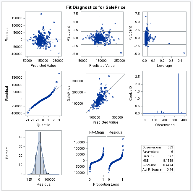
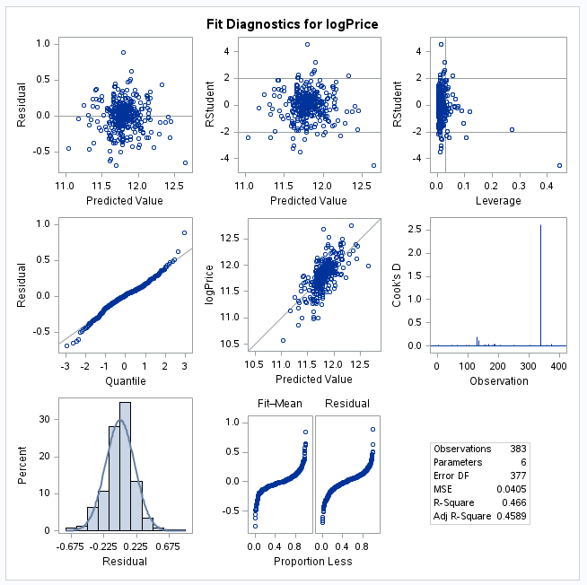
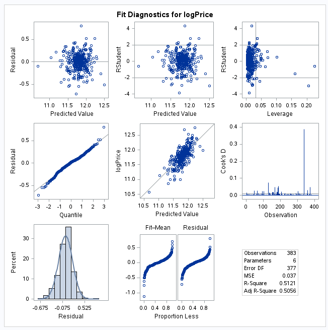
The assumptions of a linear regression model are as follows: linearity, normality, constant variance, and independence. We will address these assumptions using the Fit Diagnostics plot in Appendix D.
We can tell the data follows a linear model by looking at the Residual v Quantile plot (second row, first column). If the graph follows a diagonal line then the model will be a good linear fit. This plot shows that the linearity assumption is met.
Normality is met when the histogram of the data follows a normal distribution. The Percent v Residual plot (third row, first column) shows that this data is normally distributed and follows the normal bell curve.
Constant variance can be shown in the Residual v Predicted and the RStudent v Predicted plots (first row, first and second columns). If the data shows a random plot of points with no trends, then the data will have constant variance. Our plots below show that there is no pattern in the Residuals so this assumption is met.
Independence refers to independence of variables and independence of individual data points. Since this data is based off of the houses sold by Century 21 in Ames, we will have to assume that independence is met.
We do have two highly influential observations of large houses sold in the Edwards neighborhood for relatively low prices. While these points are highly influential, we see no reason to believe they are not a part of the population of homes sold in Ames that we are studying, therefore these outliers will be left in the analysis. These points primarily affect the indicator term for the Edwards neighborhood.
In order to compare the neighborhoods and sale price with the square footage of the living area, we looked at 4 models. We will refer to these models by their number when comparing later in the paper.
The assumptions were examined for each model, as well as other factors such as Adjusted R^2 and CV Press. The plots of each model assumption are seen, respectively in Appendices A-D.
Model Number | Adj R^2 | Assumptions Met? |
1 | 0.44 | No - linearity not met |
2 | .4587 | No - linearity not met |
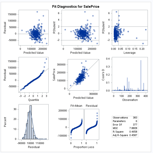
3 | .4589 | Yes -all |
4 | .5056 | Yes - all |
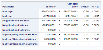
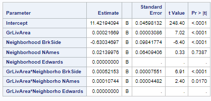
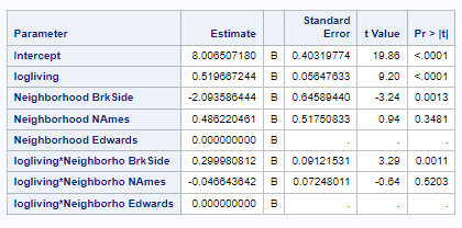
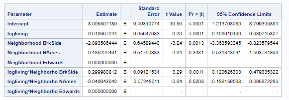
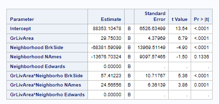
We chose the 4th model of log(Sale Price) = log(GrLivArea) * Neighborhood as it produced the highest Adj R^2 and lowest CV Press. The estimate of the sales price ends up with two different models based on the neighborhoods. There is no significant difference in the price of a house in Edwards and North Ames but there is a difference in Brookside.
Our models are:
North Ames and Edwards-
Predicted Log(SalePrice) = 8.0065 + 0.5197*log(GrLivArea)
Brookside-
Predicted Log(SalePrice) = 8.4927 + .8197*log(GrLivArea)
North Ames and Edwards: A doubling of the square footage of a living area is associated with a multiplicative change of 2^.5197 = 1.433 increase in the median Sale Price for the North Ames and Edwards neighborhoods. We are 95% certain that the multiplicative increase is in the range of (1.3274, 1.5483).
Brookside: A doubling of the square footage of a living area is associated with a multiplicative change of 2^.8197 = 1.765 increase in the median Sale Price for the Brookside neighborhood. We are 95% certain that the true multiplicative increase is in the range (1.5586, 1.9986).
https://josh-turk.shinyapps.io/StatProject-AmesHousing/
Century 21 Ames is looking to find the best model to accurately predict Sale Price of a house using the data they have collected. They want J&R to come up with four models using techniques covered in 6371 and give them the best model of the four.
Predictive Model | Adjusted R^2 | CV PRESS | Kaggle Score |
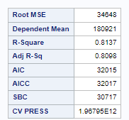
Forward | 0.8098 | 1.853E12 | .17502 |
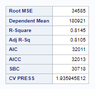
Backward | 0.8137 | 1.920E12 | .17502 |
Stepwise | 0.8098 | 1.843E12 | .17502 |
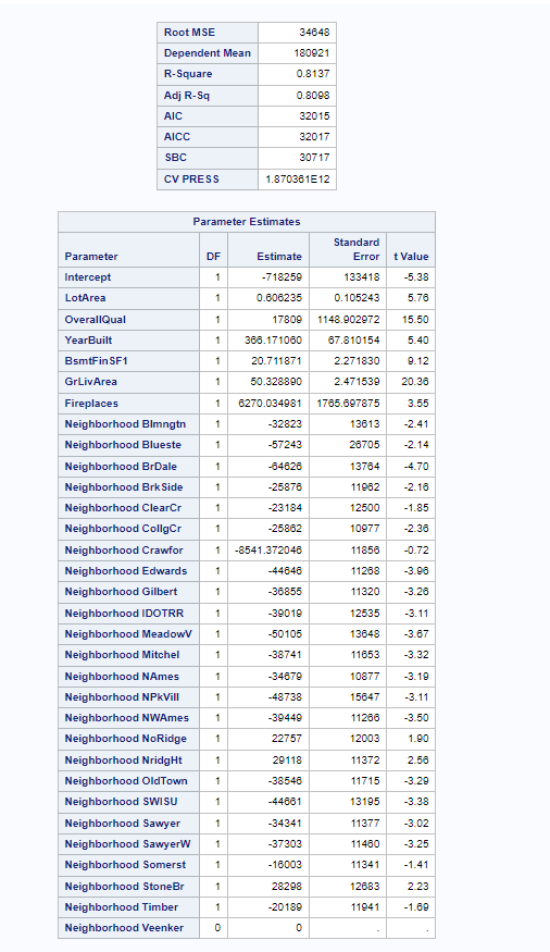
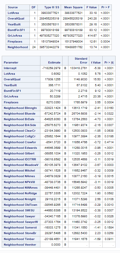
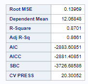
Custom | 0.8661 | 20.45173 | .16353 |
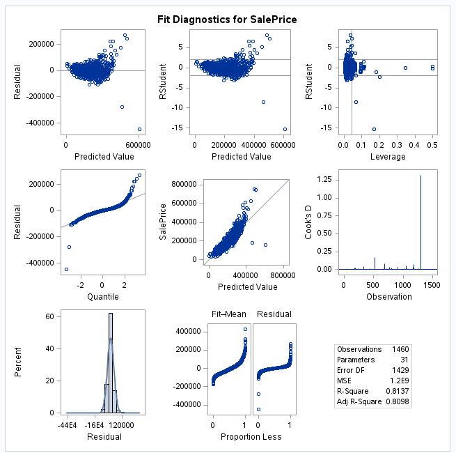
Using the techniques that we have learned has resulted in all three (Forward, Backward, and Stepwise) models having the same predictors. This will allow us to look at the assumptions using the same plots as seen in Appendix I.
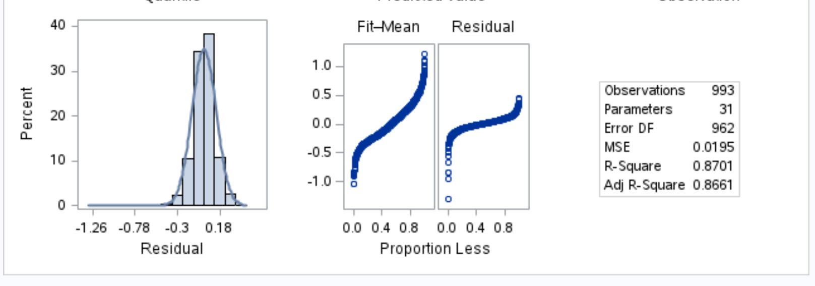
Normality is highly violated in the histogram plot because the data is left skewed. Constant variance is not met because both residual plots have a U-shaped pattern. Linearity is not met because the data doesn’t follow a linear trend.
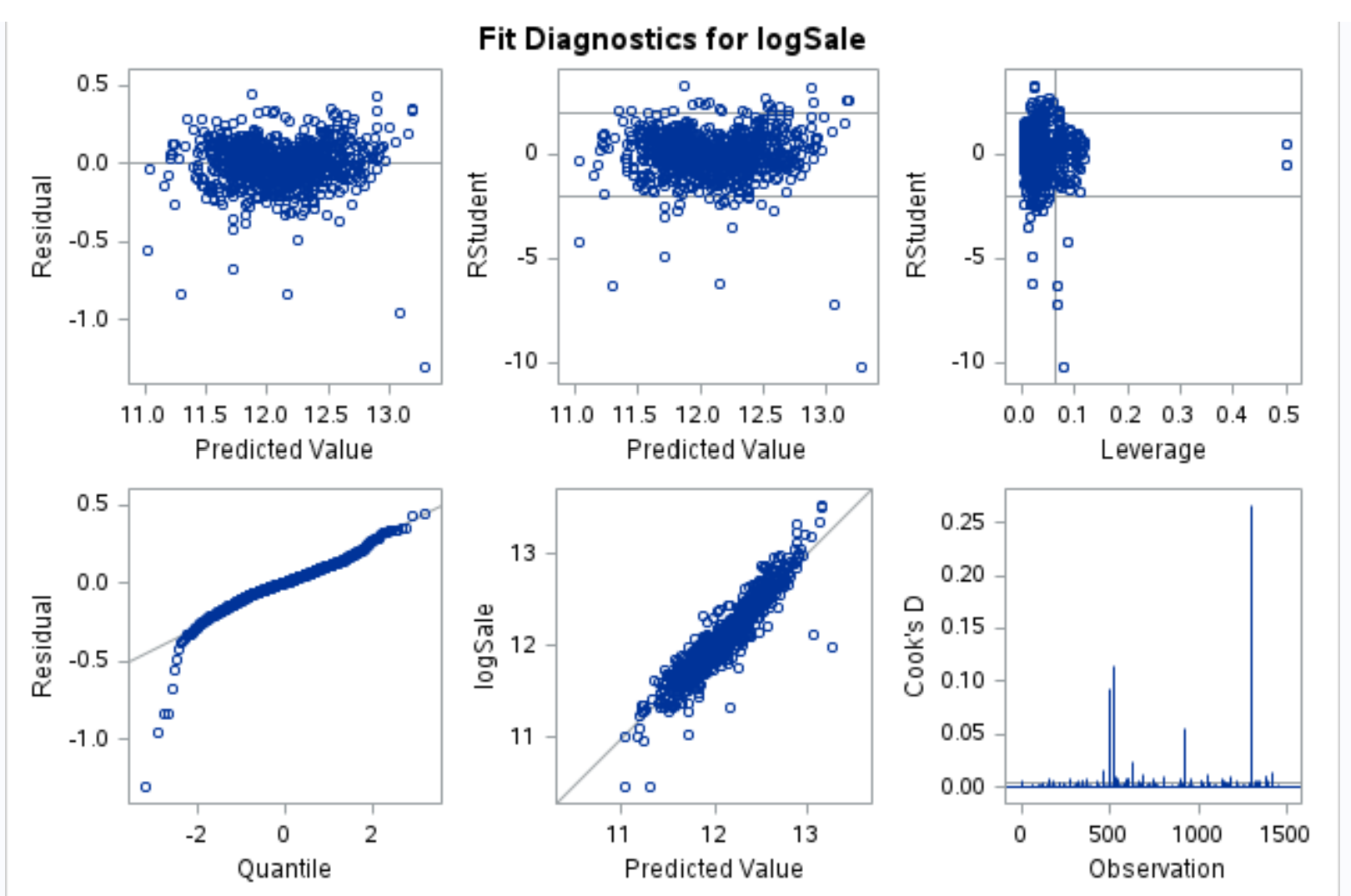
The custom model shows that the data looks more normal compared to the forward, backward, and stepwise model. There is a slight tail on this which may be due to some outliers.Constant variance is met based on the residual plots having a random pattern. We will proceed with caution on the linearity assumption as it is not 100% met.
Again we have two highly influential outliers where large houses were sold for significantly less than would otherwise be predicted. We have decided to leave these observations in as we have no reason to believe that these houses are not a part of the population of interest.
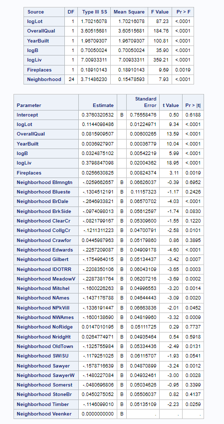
In conclusion, after running a thorough analysis, we have decided to use the custom model containing: Lot Area, Overall Quality, Year Built, Basement Finished Square feet, Living Area, Fireplaces, and Neighborhood. This model had the smallest Adjusted R^2, CV Press, and kaggle score. Out of all the models, this one will provide us with the best estimate of Sale Price in the Ames neighborhoods.
https://rachelliercke.github.io/
https://www.kaggle.com/competitions/house-prices-advanced-regression-techniques/overview
*create log variables;
data Ames2;
set Ames;
logliving = log(GrLivArea);
logPrice = log(SalePrice);
*Model 1;
proc glm data = Ames2 plots=all;
class Neighborhood (ref = "Edwards");
model SalePrice = GrLivArea | Neighborhood / solution;
run;
*Model 2;
proc glm data = Ames2 plots=all;
class Neighborhood (ref = "Edwards");
model SalePrice = logliving | Neighborhood / solution;
run;
*Model 3;
proc glm data = Ames2 plots=all;
class Neighborhood (ref = "Edwards");
model logPrice = GrLivArea | Neighborhood / solution;
run;
*Model 4;
**double log is best;
proc glm data = Ames2 plots=all;
class Neighborhood (ref = "Edwards");
model logPrice = logliving | Neighborhood / solution clparm;
run;
proc reg data = import1;
model SalePrice = MSSubClass LotArea OverallQual OverallCond YearBuilt YearRemodAdd
BsmtFinSF1 BsmtUnfSF TotalBsmtSF fstFlrSF sndFlrSF
LowQualFinSF GrLivArea BsmtFullBath BsmtHalfBath FullBath HalfBath BedroomAbvGr KitchenAbvGr TotRmsAbvGrd
Fireplaces GarageCars GarageArea WoodDeckSF
MiscVal MoSold / selection = stepwise slentry = 0.05 adjrsq;
run;
/* backward */
proc glm data = import1;
class Neighborhood BldgType;
model SalePrice = MSSubClass LotArea OverallQual OverallCond YearBuilt BsmtFinSF1
GrLivArea BsmtFullBath BedroomAbvGr KitchenAbvGr TotRmsAbvGrd Fireplaces
GarageCars ;
run;
/* stepwise */
proc reg data = import1;
model SalePrice = MSSubClass LotArea OverallQual OverallCond YearBuilt YearRemodAdd
BsmtFinSF1 BsmtUnfSF TotalBsmtSF fstFlrSF sndFlrSF
LowQualFinSF GrLivArea BsmtFullBath BsmtHalfBath FullBath HalfBath BedroomAbvGr KitchenAbvGr TotRmsAbvGrd
Fireplaces GarageCars GarageArea WoodDeckSF OpenPorchSF EnclosedPorch ScreenPorch
PoolArea MiscVal MoSold / selection = stepwise slentry = 0.1 slstay = 0.1 adjrsq;
run;
proc glmselect data = import1;
class Neighborhood MSZoning BldgType HouseStyle RoofStyle GarageType SaleCondition;
model SalePrice = MSSubClass LotArea OverallQual OverallCond YearBuilt YearRemodAdd
BsmtFinSF1 BsmtUnfSF TotalBsmtSF fstFlrSF sndFlrSF
LowQualFinSF GrLivArea BsmtFullBath BsmtHalfBath FullBath HalfBath BedroomAbvGr KitchenAbvGr TotRmsAbvGrd
Fireplaces GarageCars GarageArea WoodDeckSF OpenPorchSF EnclosedPorch
PoolArea MiscVal MoSold Neighborhood MSZoning BldgType HouseStyle RoofStyle GarageType SaleCondition
/ selection = Stepwise(stop = CV) cvmethod = random(10) stats = adjrsq;
run;
proc glmselect data = import1;
class Neighborhood MSZoning BldgType HouseStyle RoofStyle GarageType SaleCondition;
model SalePrice = MSSubClass LotArea OverallQual OverallCond YearBuilt YearRemodAdd
BsmtFinSF1 BsmtUnfSF TotalBsmtSF fstFlrSF sndFlrSF
LowQualFinSF GrLivArea BsmtFullBath BsmtHalfBath FullBath HalfBath BedroomAbvGr KitchenAbvGr TotRmsAbvGrd
Fireplaces GarageCars GarageArea WoodDeckSF OpenPorchSF EnclosedPorch
PoolArea MiscVal MoSold Neighborhood MSZoning BldgType HouseStyle RoofStyle GarageType SaleCondition
/ selection = Backward(stop = CV) cvmethod = random(10) stats = adjrsq;
run;
proc glmselect data = import1;
class Neighborhood MSZoning BldgType HouseStyle RoofStyle GarageType SaleCondition;
model SalePrice = MSSubClass LotArea OverallQual OverallCond YearBuilt YearRemodAdd
BsmtFinSF1 BsmtUnfSF TotalBsmtSF fstFlrSF sndFlrSF
LowQualFinSF GrLivArea BsmtFullBath BsmtHalfBath FullBath HalfBath BedroomAbvGr KitchenAbvGr TotRmsAbvGrd
Fireplaces GarageCars GarageArea WoodDeckSF OpenPorchSF EnclosedPorch
PoolArea MiscVal MoSold Neighborhood MSZoning BldgType HouseStyle RoofStyle GarageType SaleCondition
/ selection = Forward(stop = CV) cvmethod = random(10) stats = adjrsq;
run;
proc glm data = import1 plots=all;
model SalePrice = MSSubClass LotArea OverallQual OverallCond YearBuilt
BsmtFinSF1 GrLivArea BedroomAbvGr GarageCars / solution;
run;
data Ames4;
set import1;
logSale = log(SalePrice);
run;
proc print data = Ames4;
run;
proc glm data = Ames4 plots=all;
model logSale = MSSubClass LotArea OverallQual OverallCond YearBuilt
BsmtFinSF1 GrLivArea BedroomAbvGr GarageCars / solution;
run;
data importSec;
set import1;
logLot = log(LotArea);
logSale = log(SalePrice);
logB = log(BsmtFinSF1);
logLiv = log(GrLivArea);
run;
proc reg data = importSec;
model logSale = logLot OverallQual YearBuilt logB
GrLivArea BedroomAbvGr Fireplaces
GarageCars / vif tol;
run;
proc glm data = importSec plots=all;
class Neighborhood;
model logSale = logLot OverallQual YearBuilt logB
GrLivArea BedroomAbvGr Fireplaces Neighborhood/ solution;
run;
proc glmselect data = import1;
class Neighborhood;
model SalePrice = LotArea OverallQual YearBuilt BsmtFinSF1
GrLivArea BedroomAbvGr Fireplaces Neighborhood
/ selection = Forward(stop = CV) cvmethod = random(10) stats = adjrsq;
run;
proc glmselect data = import1;
class Neighborhood;
model SalePrice = LotArea OverallQual YearBuilt BsmtFinSF1
GrLivArea BedroomAbvGr Fireplaces Neighborhood
/ selection = Backward(stop = CV) cvmethod = random(10) stats = adjrsq;
run;
proc glmselect data = import1;
class Neighborhood;
model SalePrice = LotArea OverallQual YearBuilt BsmtFinSF1
GrLivArea BedroomAbvGr Fireplaces Neighborhood
/ selection = Stepwise(stop = CV) cvmethod = random(10) stats = adjrsq;
run;
*Forward model with p-vals;
proc glm data = import1 plots = ALL;
class Neighborhood;
model SalePrice = LotArea OverallQual YearBuilt BsmtFinSF1
GrLivArea Fireplaces Neighborhood / solution;
run;
proc glmselect data = importSec;
class Neighborhood;
model logSale = logLot OverallQual YearBuilt logB
logLiv Fireplaces Neighborhood/ selection = Stepwise(stop=CV) cvmethod = random(10) stats = adjrsq;
run;
proc glm data = importSec plots=all;
class Neighborhood;
model logSale = logLot OverallQual YearBuilt logB
logLiv Fireplaces Neighborhood/ solution;
run;